Autoencoders

Autoencoders

An Autoencoder (AE) is a type of neural network that learns to compress (encode) and reconstruct (decode) data. It is used for dimensionality reduction, anomaly detection, and feature learning without requiring labeled data.

How Does It Work?

An autoencoder consists of two main parts:

1. Encoder: Compresses input into a lower-dimensional latent representation (also called bottleneck).
2. Decoder: Reconstructs the original input from the compressed representation.

This process forces the model to learn the most important features of the input data.

Mathematical Formulation

Given an input X, the autoencoder transforms it as follows:

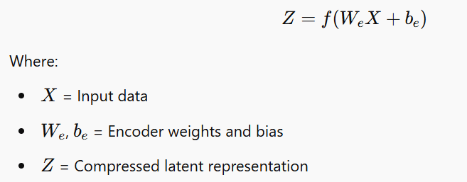
1️⃣ Encoding Function:

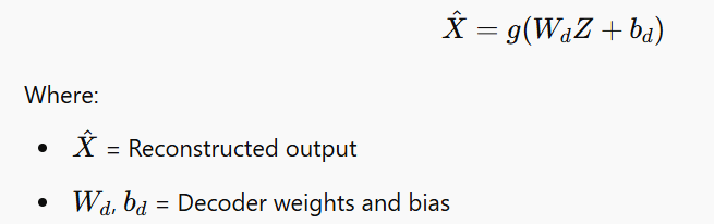
2️⃣ Decoding Function:

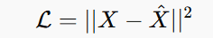
3️⃣ Loss Function:

This measures the difference between the input and the reconstructed output. The goal is to minimize this loss so that X^ is as close to X as possible.

Autoencoder: A Real-Life Example with Mathematical Explanation

Real-Life Scenario: Image Compression

Let’s say we have a high-resolution black-and-white image of size 1000 × 1000 pixels, meaning we have 1,000,000 pixels (features). Storing these large images takes up a lot of memory. Autoencoders help by reducing the number of features while preserving the image quality.

---

Step-by-Step Mathematical Explanation

Step 1: Representing the Image as a Matrix

A grayscale image of size 1000×1000 is represented as a matrix X where each element Xi,j​ is a pixel intensity (0 = black, 255 = white).

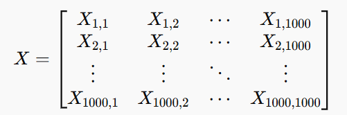
Since we have 1,000,000 pixels, an autoencoder will reduce this high-dimensional data into a compressed form (latent space representation).

---

Step 2: Encoding – Reducing Dimensionality

The encoder reduces the 1,000,000-dimensional input into a lower-dimensional representation, say 100 features. This is done using a weight matrix We and a bias term be:

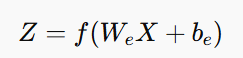
Where:

• X is the original image matrix
• We is the weight matrix for encoding
• be​ is the bias
• f is an activation function (e.g., ReLU, Sigmoid)
• Z is the latent representation (compressed image)

If X was 1000 × 1000 (1,000,000 features), now Z might be 100 × 1 (only 100 features).

Step 3: Decoding – Reconstructing the Image

The decoder reconstructs the image from the compressed representation:

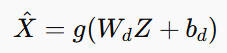
Where:

• Wd​ is the weight matrix for decoding
• bd​ is the bias
• g is an activation function (e.g., ReLU, Sigmoid)
• X^ is the reconstructed image

🔹 This reconstructed image should be similar to the original but uses much less storage.

Step 4: Loss Function – Measuring the Reconstruction Quality

To ensure that the reconstructed image (X^) is close to the original (X), we minimize the Mean Squared Error (MSE) Loss:

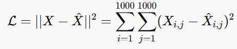
The goal is to make the reconstructed image as similar as possible to the original.

Final Output: Compressed & Reconstructed Image

✅ Original Image: 1,000,000 features
✅ Compressed Representation (Latent Space): 100 features
✅ Reconstructed Image: Uses only 100 features but still looks like the original

Real-World Applications

1️⃣ JPEG Image Compression – Similar to how JPEG reduces image size while preserving quality.
2️⃣ Denoising Images – Autoencoders can remove noise while keeping the important details.
3️⃣ Anomaly Detection – Detect fraudulent transactions by learning normal patterns and flagging anomalies.

Python implementation of an Autoencoder for image compression using the MNIST dataset (handwritten digits). It uses TensorFlow/Keras to train an autoencoder and visualize the results.

---

Steps in the Code

1️⃣ Load the MNIST dataset (28×28 grayscale images).
2️⃣ Build the encoder (reduces 28×28 to a lower-dimensional representation).
3️⃣ Build the decoder (reconstructs the image from the compressed form).
4️⃣ Train the model.
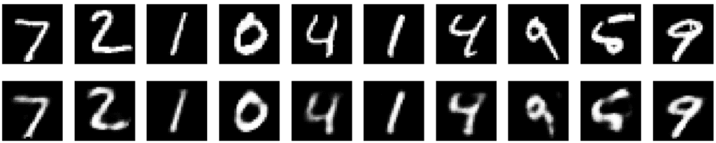
5️⃣ Visualize original vs. reconstructed images.

import tensorflow as tf
from tensorflow import keras
from tensorflow.keras.layers import Input, Dense, Flatten, Reshape
import matplotlib.pyplot as plt
import numpy as np

# Load MNIST dataset
(x_train, _), (x_test, _) = keras.datasets.mnist.load_data()

# Normalize data to range [0,1]
x_train, x_test = x_train / 255.0, x_test / 255.0

# Flatten images (28x28 -> 784)
x_train = x_train.reshape(-1, 784)
x_test = x_test.reshape(-1, 784)

# Define the Autoencoder
encoding_dim = 32  # Size of compressed representation

# Encoder
input_img = Input(shape=(784,))
encoded = Dense(128, activation='relu')(input_img)
encoded = Dense(64, activation='relu')(encoded)
encoded = Dense(encoding_dim, activation='relu')(encoded)

# Decoder
decoded = Dense(64, activation='relu')(encoded)
decoded = Dense(128, activation='relu')(decoded)
decoded = Dense(784, activation='sigmoid')(decoded)  # Output same shape as input

autoencoder = keras.Model(input_img, decoded)
autoencoder.compile(optimizer='adam', loss='mse')

# Train the autoencoder
autoencoder.fit(x_train, x_train, epochs=10, batch_size=256, shuffle=True, validation_data=(x_test, x_test))

# Encode and decode some test images
encoded_imgs = autoencoder.predict(x_test)

# Plot original vs. reconstructed images
def plot_images(original, reconstructed, n=10):
    plt.figure(figsize=(20, 4))
    for i in range(n):
        # Original
        ax = plt.subplot(2, n, i + 1)
        plt.imshow(original[i].reshape(28, 28), cmap='gray')
        plt.axis('off')
        
        # Reconstructed
        ax = plt.subplot(2, n, i + 1 + n)
        plt.imshow(reconstructed[i].reshape(28, 28), cmap='gray')
        plt.axis('off')
    plt.show()

plot_images(x_test, encoded_imgs)

Output

Explanation of the Code

✅ Loads the MNIST dataset and normalizes it.
✅ Defines an encoder (784 → 32 features).
✅ Defines a decoder (32 → 784 features).
✅ Trains the autoencoder for image reconstruction.
✅ Visualizes original vs. reconstructed images.