Private: AI Unleashed: Mastering AI at Your Pace

0 of 24 lessons complete (0%)

Neural Network

Neural Network

You don’t have access to this lesson

Please register or sign in to access the course content.

Introduction

Neural networks are the backbone of modern artificial intelligence, enabling machines to perform tasks that once required human intelligence. This guide will take you through the fundamental concepts of neural networks, their types, how they learn, and their practical applications. We’ll also provide implementation examples in Python.

1. Basic Components of a Neural Network

Neurons

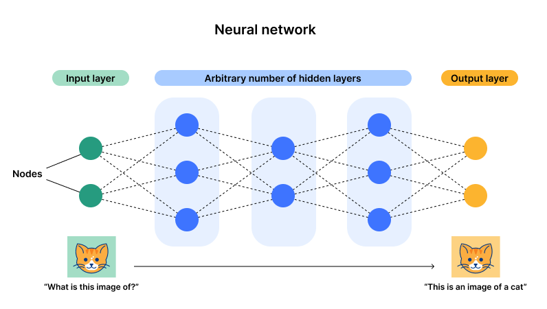
A neuron is the basic building block of a neural network. Each neuron receives inputs, processes them, and produces an output. The processing is done using a weighted sum of the inputs, followed by an activation function.

Layers

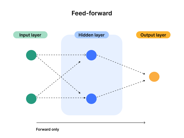
  • Input Layer: This layer receives the initial data and passes it to the next layer.
  • Hidden Layers: These layers perform complex computations and feature extraction.
  • Output Layer: This layer produces the final output of the network.

Weights and Biases

Weights are parameters that determine the importance of each input. Biases are additional parameters that adjust the output along with the weights.

Activation Functions

Activation functions introduce non-linearity into the model, allowing it to learn complex patterns. Common activation functions include:

  • Sigmoid: σ(x)=11+e−x\sigma(x) = \frac{1}{1 + e^{-x}}σ(x)=1+e−x1​
  • Tanh: tanh⁡(x)=ex−e−xex+e−x\tanh(x) = \frac{e^x – e^{-x}}{e^x + e^{-x}}tanh(x)=ex+e−xex−e−x​
  • ReLU: ReLU(x)=max⁡(0,x)\text{ReLU}(x) = \max(0, x)ReLU(x)=max(0,x)
2. Types of Neural Networks

In feedforward neural networks, the data moves in one direction—from the input layer to the output layer—without cycles or loops. We’ll use a feedforward neural network to predict house prices based on features like the number of bedrooms, square footage, and age of the house.

##Feedforward Neural Network: Predicting House Prices

import numpy as np
from sklearn.model_selection import train_test_split
from sklearn.preprocessing import StandardScaler
import tensorflow as tf
from tensorflow.keras import layers, models

# Generate synthetic house price data
np.random.seed(42)
num_samples = 1000
square_footage = np.random.randint(500, 3500, num_samples)
num_bedrooms = np.random.randint(1, 5, num_samples)
age_of_house = np.random.randint(0, 100, num_samples)
prices = square_footage * 300 + num_bedrooms * 5000 + age_of_house * 200 + np.random.randint(-10000, 10000, num_samples)

# Combine features into a single array
features = np.column_stack((square_footage, num_bedrooms, age_of_house))

# Split data into training and testing sets
X_train, X_test, y_train, y_test = train_test_split(features, prices, test_size=0.2, random_state=42)

# Standardize the data
scaler = StandardScaler()
X_train = scaler.fit_transform(X_train)
X_test = scaler.transform(X_test)

# Build the feedforward neural network
model = models.Sequential([
    layers.Dense(64, activation='relu', input_shape=(3,)),
    layers.Dense(64, activation='relu'),
    layers.Dense(1)
])

model.compile(optimizer='adam', loss='mse')

# Train the model
model.fit(X_train, y_train, epochs=50, batch_size=32, validation_split=0.2)

# Evaluate the model
loss = model.evaluate(X_test, y_test)
print("Mean Squared Error on Test Data:", loss)

# Predict house prices
predictions = model.predict(X_test[:5])
print("Predicted Prices:", predictions)
print("Actual Prices:", y_test[:5])

CNNs are specialized for processing grid-like data, such as images. They use convolutional layers to extract features and pooling layers to reduce dimensionality. We’ll use a CNN to classify handwritten digits from the MNIST dataset.

##Classifying Handwritten Digits

import tensorflow as tf
from tensorflow.keras import layers, models
from tensorflow.keras.datasets import mnist
import matplotlib.pyplot as plt

# Load and preprocess the MNIST dataset
(X_train, y_train), (X_test, y_test) = mnist.load_data()
X_train = X_train.reshape((60000, 28, 28, 1)).astype('float32') / 255
X_test = X_test.reshape((10000, 28, 28, 1)).astype('float32') / 255

# Build the CNN model
model = models.Sequential([
    layers.Conv2D(32, (3, 3), activation='relu', input_shape=(28, 28, 1)),
    layers.MaxPooling2D((2, 2)),
    layers.Conv2D(64, (3, 3), activation='relu'),
    layers.MaxPooling2D((2, 2)),
    layers.Flatten(),
    layers.Dense(64, activation='relu'),
    layers.Dense(10, activation='softmax')
])

model.compile(optimizer='adam', loss='sparse_categorical_crossentropy', metrics=['accuracy'])

# Train the model
model.fit(X_train, y_train, epochs=5, batch_size=64, validation_split=0.1)

# Evaluate the model
test_loss, test_acc = model.evaluate(X_test, y_test)
print("Test Accuracy:", test_acc)

# Predict on test images
predictions = model.predict(X_test[:5])
print("Predicted Labels:", np.argmax(predictions, axis=1))
print("Actual Labels:", y_test[:5])

# Plot some test images with their predicted labels
for i in range(5):
    plt.imshow(X_test[i].reshape(28, 28), cmap='gray')
    plt.title(f"Predicted: {np.argmax(predictions[i])}, Actual: {y_test[i]}")
    plt.show()

RNNs are designed for sequential data, like time series or natural language. They have loops that allow information to persist. We’ll use an RNN to predict stock prices based on historical data.

Example: Predicting Stock Prices

##Predicting Stock Prices

import numpy as np
import pandas as pd
import matplotlib.pyplot as plt
from sklearn.preprocessing import MinMaxScaler
import tensorflow as tf
from tensorflow.keras import layers, models

# Generate synthetic stock price data
np.random.seed(42)
dates = pd.date_range(start='2020-01-01', periods=100)
prices = np.sin(np.linspace(0, 10, 100)) + np.random.normal(0, 0.1, 100) + np.linspace(10, 20, 100)

# Create a DataFrame
data = pd.DataFrame({'Date': dates, 'Price': prices})
data.set_index('Date', inplace=True)

# Normalize the data
scaler = MinMaxScaler()
data['Price'] = scaler.fit_transform(data['Price'].values.reshape(-1, 1))

# Create sequences for RNN input
def create_sequences(data, seq_length):
    X, y = [], []
    for i in range(len(data) - seq_length):
        X.append(data[i:i+seq_length])
        y.append(data[i+seq_length])
    return np.array(X), np.array(y)

seq_length = 10
X, y = create_sequences(data['Price'].values, seq_length)

# Split data into training and testing sets
X_train, X_test = X[:80], X[80:]
y_train, y_test = y[:80], y[80:]

# Build the RNN model
model = models.Sequential([
    layers.SimpleRNN(50, activation='relu', input_shape=(seq_length, 1)),
    layers.Dense(1)
])

model.compile(optimizer='adam', loss='mse')

# Train the model
model.fit(X_train, y_train, epochs=20, batch_size=8)

# Predict on test data
predictions = model.predict(X_test)

# Rescale predictions back to original scale
predictions = scaler.inverse_transform(predictions)
y_test = scaler.inverse_transform(y_test.reshape(-1, 1))

# Plot the results
plt.plot(dates[-20:], y_test, label='Actual Prices')
plt.plot(dates[-20:], predictions, label='Predicted Prices')
plt.xlabel('Date')
plt.ylabel('Price')
plt.legend()
plt.show()

We’ll use a GAN to generate new handwritten digits similar to those in the MNIST dataset.

import numpy as np
import tensorflow as tf
from tensorflow.keras import layers, models
from tensorflow.keras.datasets import mnist
import matplotlib.pyplot as plt

# Load and preprocess the MNIST dataset
(X_train, _), (_, _) = mnist.load_data()
X_train = X_train.reshape((60000, 28, 28, 1)).astype('float32') / 255

# Build the generator
def build_generator():
    model = models.Sequential([
        layers.Dense(256, activation='relu', input_dim=100),
        layers.BatchNormalization(),
        layers.Dense(512, activation='relu'),
        layers.BatchNormalization(),
        layers.Dense(1024, activation='relu'),
        layers.BatchNormalization(),
        layers.Dense(28 * 28 * 1, activation='sigmoid'),
        layers.Reshape((28, 28, 1))
    ])
    return model

# Build the discriminator
def build_discriminator():
    model = models.Sequential([
        layers.Flatten(input_shape=(28, 28, 1)),
        layers.Dense(512, activation='relu'),
        layers.Dense(256, activation='relu'),
        layers.Dense(1, activation='sigmoid')
    ])
    return model

generator = build_generator()
discriminator = build_discriminator()

# Compile the discriminator
discriminator.compile(optimizer='adam', loss='binary_crossentropy', metrics=['accuracy'])

# Build and compile the GAN
discriminator.trainable = False
gan_input = layers.Input(shape=(100,))
gan_output = discriminator(generator(gan_input))
gan = models.Model(gan_input, gan_output)
gan.compile(optimizer='adam', loss='binary_crossentropy')

# Training the GAN
def train_gan(generator, discriminator, gan, epochs=10000, batch_size=64):
    for epoch in range(epochs):
        # Train the discriminator
        real_images = X_train[np.random.randint(0, X_train.shape[0], batch_size)]
        fake_images = generator.predict(np.random.normal(0, 1, (batch_size, 100)))

        real_labels = np.ones((batch_size, 1))
        fake_labels = np.zeros((batch_size, 1))

        d_loss_real = discriminator.train_on_batch(real_images, real_labels)
        d_loss_fake = discriminator.train_on_batch(fake_images, fake_labels)
        d_loss = 0.5 * np.add(d_loss_real, d_loss_fake)

        # Train the generator
        noise = np.random.normal(0, 1, (batch_size, 100))
        valid_y = np.ones((batch_size, 1))

        g_loss = gan.train_on_batch(noise, valid_y)

        # Print the progress
        if epoch % 1000 == 0:
            print(f"{epoch} [D loss: {d_loss[0]} | D accuracy: {100 * d_loss[1]}] [G loss: {g_loss}]")

train_gan(generator, discriminator, gan)

# Generate new handwritten digits
def generate_images(generator, num_images=5):
    noise = np.random.normal(0, 1, (num_images, 100))
    generated_images = generator.predict(noise)
    generated_images = generated_images.reshape((num_images, 28, 28))

    for i in range(num_images):
        plt.imshow(generated_images[i], cmap='gray')
        plt.show()

generate_images(generator)


3. How Neural Networks Learn

Forward Propagation

During forward propagation, the input data passes through the network layers, and the initial output is generated. We’ll use a feedforward neural network to predict house prices based on features like the number of bedrooms, square footage, and age of the house.

Loss Function

The loss function measures the difference between the predicted output and the actual output. Common loss functions include mean squared error (MSE) and categorical cross-entropy.

Backpropagation

Backpropagation adjusts the weights and biases to minimize the loss function. It calculates the gradient of the loss with respect to each weight by the chain rule, propagating the error backward.

Optimization Algorithms

Optimization algorithms like Gradient Descent are used to update the weights and biases. Variants like Stochastic Gradient Descent (SGD) and Adam are commonly used.

4. Applications of Neural Networks

Image and Speech Recognition

Neural networks are used in facial recognition systems and voice assistants, enabling devices to understand and respond to human input.

Natural Language Processing (NLP)

NLP applications include language translation, sentiment analysis, and chatbots, helping machines understand and generate human language.

Autonomous Systems

Neural networks power self-driving cars and robots, allowing them to navigate and make decisions in real-time.

Healthcare

Neural networks assist in disease prediction and medical image analysis, improving diagnostic accuracy and treatment planning.

Finance

In finance, neural networks are used for fraud detection, stock market prediction, and risk management, enhancing the decision-making process.